Simplified Energy Balance Model
Contents
Simplified Energy Balance Model#
In this exercise we will develop a simple zero-dimensional energy balance model for the Earth. With this conceptual model we will look at complex interactions in the atmosphere with simplified processes. We will show how simple model can help to derive important insights into the Earth system and how sensitivity simulations provide a deeper understanding of the observed climate variability.
Learning objectives:#
Global surface emission temperature
What is transmissivity
Equilibrium temperature
Equilibrium states in the Earth system
Greenhouse effect
Develop a simple conceptual model
Integrate a model in time
How to set up sensitivity runs
After the exercise you should be able to answer the following questions:#
Why can we run climate simulations for many decades even though our predictability of weather events is very limited?
With this model we will perform sensitivity simulations that will show us important processes in the atmosphere.
Python Notebooks#
Preliminary considerations: The global energy budget#
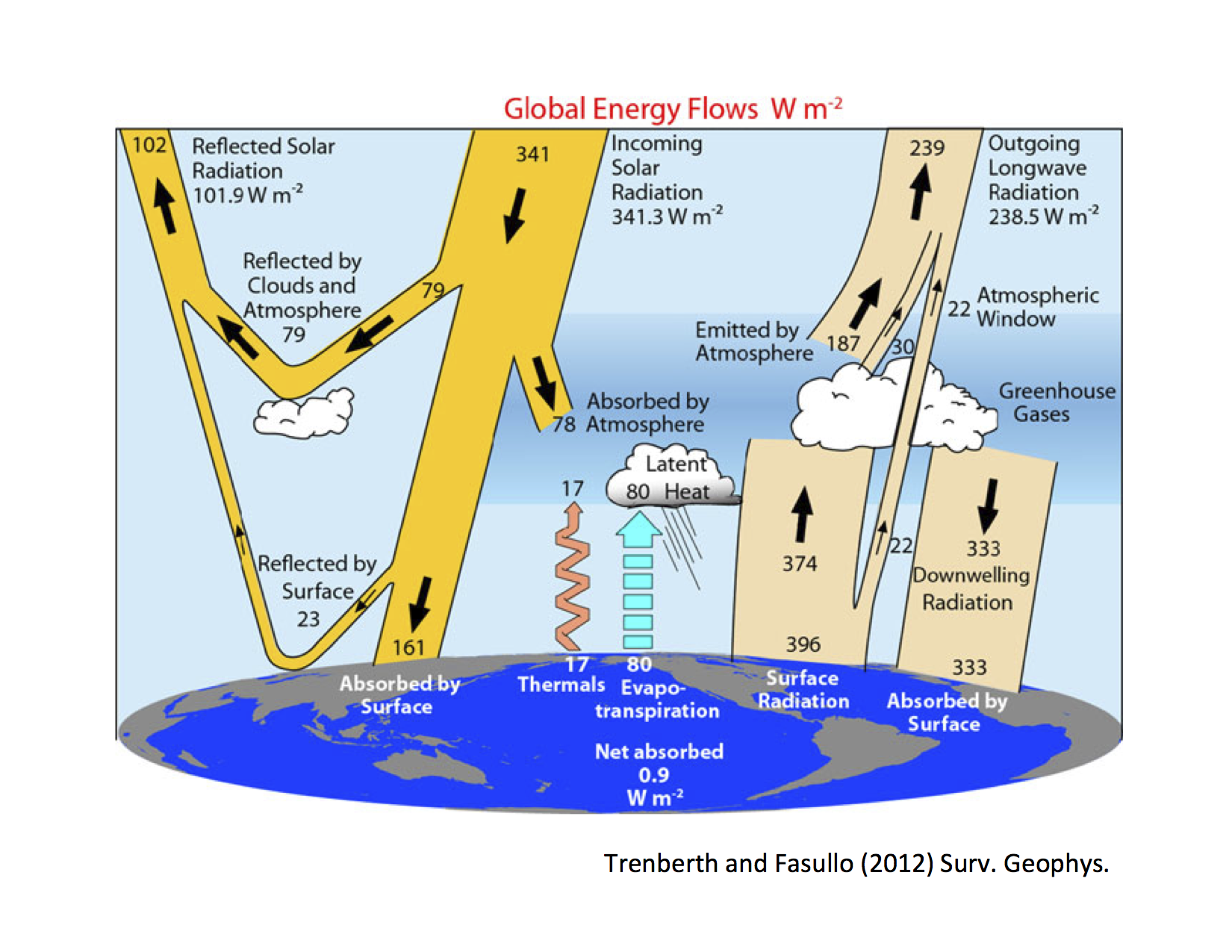
Fig. 1 Observed global energy flows (Trenberth and Fasullo (2012).#
Assume that the Earth behaves like a blackbody radiator with effective global mean surface emission temperature \(T_s\). Use the Stefan-Boltzmann law to calculate the emission temperature using the observed outgoing longwave radiation (OLR) (see Fig. 1)
with \(\sigma=5.67\cdot10^{-8}\) the Stefan=Boltzmann constant. Compare the value with the mean global surface temperature of the earth? Does the model assumption that the Earth is a blackbody radiator seem justified?
Task 1: Write a Python function for the OLR and effective temperature for later use.
The emission into space is reduced due to the greenhouse effect. We make a simplified assumption that only part of the radiation is emitted into space and part of the energy remains in the system.
Task 2: Extend the OLR function by a transmissivity constant \(\tau\) which takes this effect into account. Determine the transmissivity for a global mean temperature of 288 K.
Task 3: Determine the planetary albedo from the observations (Fig. 1) and write a function for the absorbed shortwave radiation (ASR), the part of the incoming sunlight that is not reflected back to space.
Task 4: What additional amount of energy would have to remain in the system for the global temperature to rise by 4 K?
Before we turn to a time-dependent energy balance model, we want to deal with the concept of equilibrium temperature. It is based on the fundamental assumption that the energy balance in the Earth system is balanced, i.e.
This condition can only be fulfilled if there is a corresponding equilibrium temperature that ensures that the OLR balances the short-wave radiation balance. It follows that
Task 5: Rearrange Eq (2) for the temperature denoting our equilibrium temperature. Substitute the observed values for insolation, transmissivity and planetary albedo and calculate the equlibrium temperature.
Task 6: Conceptual approaches, such as equilibrium temperature, can be used to calculate simple scenarios like the relationship between the increase in albedo due to increased cloud cover and the associated decrease in transmissivity. For example, assume that the planetary albedo increases to 0.32 due to more cloud cover and that the transmissivity decreases to 0.57. What would be the new equilibrium temperature?
Simple Energy Balance Model: Problem description#
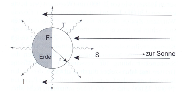
Fig. 2 Schematic of the zero-dimensional Energy Balance Model.#
Natural processes always counteract disturbances in order to stabilise the system that has been brought out of equilibrium. The adjustment of the system to disturbances is not an abrupt but a transient process. The equilibrium temperature approach is therefore a theoretical approach that does not occur in nature. The Earth system has a latency period that it needs to adjust to changes in the energy balance. We now want to introduce a time-dependent zero-dimensional energy model that allows us to investigate this adjustment. A zero-dimensional energy model means that we consider the Earth as a sphere and calculate the global averaged and long-term equilibrium of radiation fluxes. Furthermore, we neglect spatial variabilities. With this simple approach, Arthenius was already able to gain good insights in the 19th century.
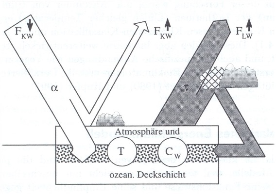
Fig. 3 Considered energy fluxes and processes.#
The energy balance is determined by the global radiation and the outgoing long-wave radiation (see Fig. 3). Part of the incoming short-wave radiation is reflected at the earth’s surface given by global albedo. According to the Stefan-Boltzmann law, the earth’s surface radiates long-wave energy. Due to the path (transmission) through the atmosphere, part of this radiation energy is absorbed and remains in the Earth system. We also assume that the surface of the Earth is uniform with a constant heat capacity and a homogeneous surface temperature.
If these assumptions are made, the change of energy in the Earth system can be described in a simplified way by
with \(dE\) the change in energy, \(C_w\) [J m\(^{-2}\) K\(^{-1}\)] the heat capacity, \(T_s\) [K] the global mean surface temperatur, ASR the absorbed shortwave radiation and OLR the outgoing longwave radiation. The term \(\frac{dT_s}{dt}\) is the rate of change of the global average surface temperature.
How to solve time dependend models?
This simple model equation is a first-order Ordinary Differential Equation (ODE) for \(T_s\) as a function of time. Under certain conditions, analytical solutions exist for this type of equation. However in many cases, these equations must or are solved numerically. We will look at how these equations are discretised at a later stage.
In general, the derivative can be approximated by a finite difference, then the above equation can be rewritten as
where \(\Delta T\) is the temperatur difference \(\Delta T=T_2-T_1\) between two discrete points in time \(\Delta t = t_2-t_1\). The \(\Delta t\) is called the timestep. Substituting the difference approach into the above equation we get
Task 7: Rearrange Eq. (5) so that you can predict future temperature.
Task 8: Write a function called step_forward(T, dt) that returns the new temperature given the old temeprature \(T\) and timestep \(dt\). Assume an initial temperature of 288 K and integrate the function for three timesteps (choose \(dt\) = 1 year) and observe how the temperature changes.
Task 9: Integrate the equation over a time of 1000 years. Use the following initial and boundary conditions: \(S_0\)=1360 W m\(^{-2}\), \(T(0)\) = 273 K, \(C_w\) = 10^8 J/(m\(^2 \cdot\) K), \(\alpha\) = 0.3, \(\tau\) = 0.61. Describe in your own words what you observe.
Task 10: What happens if the intial temperature is set to 293 K?
Task 11: What changes do you observe with a higher \(C_w\) value (e.g. \(C_w\) =10\(\cdot10^8\) J/(m\(^2 \cdot\) K)?
Task 12: How does the result change when \(\tau=1\)?
Task 13: What are the disadvantages of the energy balance model? How could it be improved?
Case study: Venus
Calculate the mean surface temperature on Venus. Due to its proximity to the Sun, Venus has a very high irradiance of \(S_{0}=2619 ~ Wm^{-2}\). Due to the high cloud cover, the albedo is about 0.7. What surface temperature can be expected? (Use the previous values for \(C_w\) and \(\tau\)).
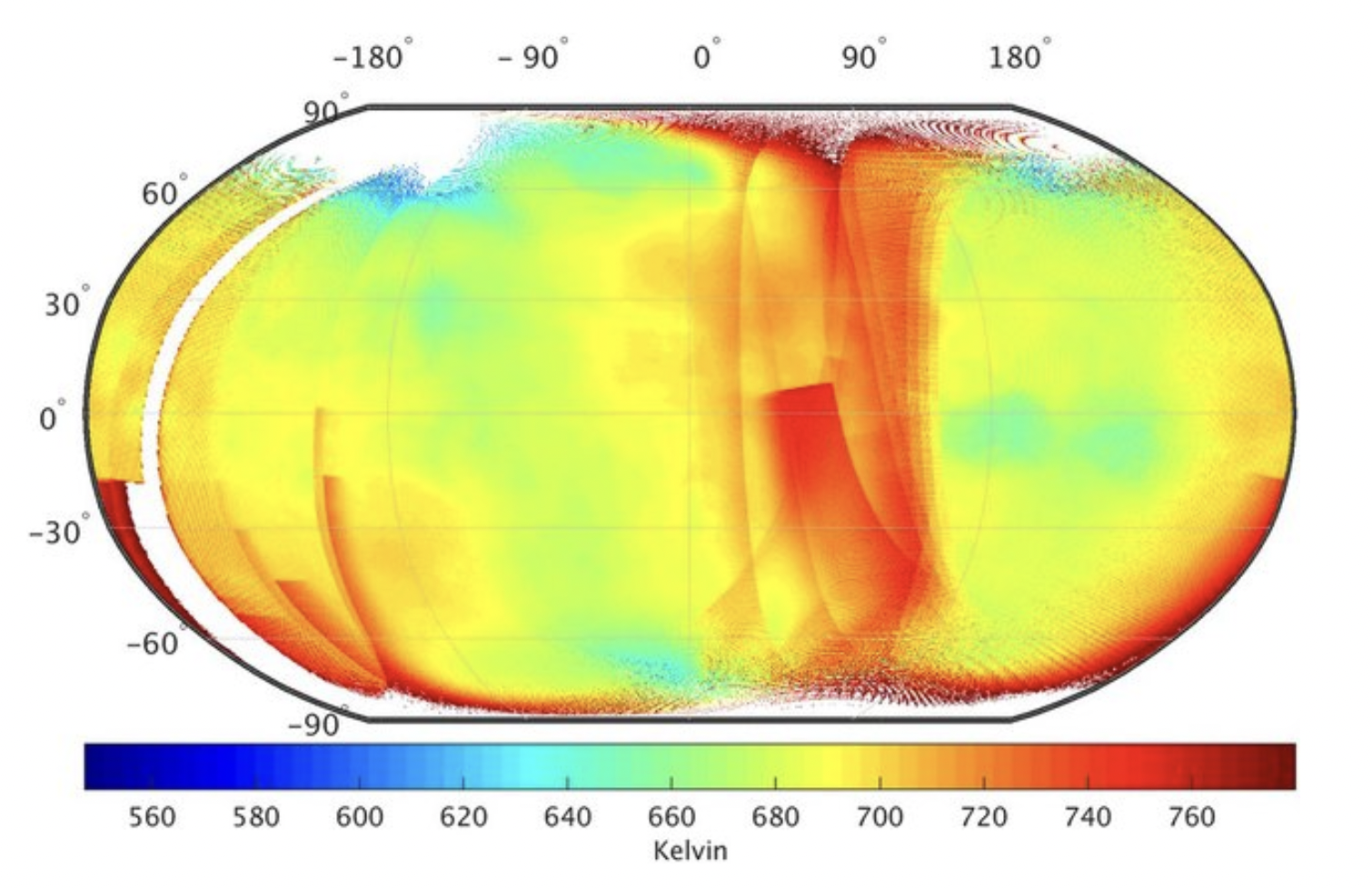
Fig. 4 Nightside surface temperature of Venus with spatial resolution of 0.5° × 0.5°. Surface temperature retrievals are based on IR1 data from Akatsuki mission between July 21, 2016 and December 7, 2016. White areas indicate either data is absent or erroneous. High altitude regions are relatively colder than low altitude regions (Data source: https://darts.jaxa.jp/planet/project/akatsuki/ir1.html.en)#
Fig. 4 shows the surface temperatures of Venus derived from IR measurements. Compare the measurements with your simulation. Is there a difference? If so, why does this difference exist.
