Von-May function
Von-May function#
Task 1: Write a function which solves the Von-May-Equation.
Problem description:
The starting point for our analysis is the ‘Von-May-Equation’, which is given by
\begin{align}
y_{t+1} = r \cdot y_{t} \cdot (1-y_{t}), \end{align}with \(r\) an pre-defined parameter and \(y\) the function value at time \(t\) and \(t+1\).
import matplotlib.pyplot as plt

def von_may(y0,r):
    '''
    y0 :: initial values
    r  :: pre-defined parameter
    '''
    # Write your code here
    yi = y0

    # result array
    result = [yi]

    # itegrate over x steps
    for t in range(500):
        # Von-May equation
        y = r * yi * (1-yi)

        # store newly calculates values to yi
        yi = y

        # append new values to result list
        result.append(y)

    return(result)
Task 2: Run the code for several initial and parameter combination. What is particularly striking about increasing r-values?
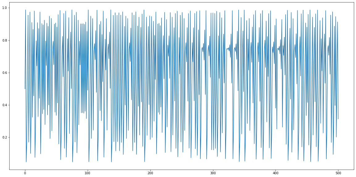
y(0)=0.5 and r=2.80 (alternatively, use y(0)=0.9)
y(0)=0.5 and r=3.30 (alternatively, use y(0)=0.9)
y(0)=0.5 and r=3.95 (alternatively, use y(0)=0.495)
y(0)=0.8 and r=2.80
# Integrate the equation and plot the results
res = von_may(0.5, 3.95)
plt.figure(figsize=(20,10))
plt.plot(res)
[<matplotlib.lines.Line2D at 0x110148460>]
Extend the Von-May function
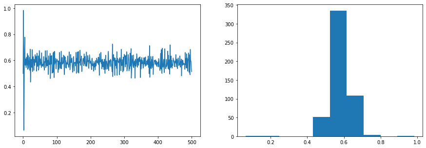
Task 3: Extend this Von-May function by generating 20 random r-values and run simulations with them. Sample the values from a normal distribution with mean 3.95 and standard deviation 0.015 (limit the r-values between 0 and 4). Then average over all time series. Plot both the time series, the averaged time series and the histogram of the averaged time series. What do you observe?
import random
import numpy as np


def ensemble_may(n, y0, r):
    """
    n :: ensemble members
    y0 :: initial value
    r :: pre-defined parameter
    """
    # Create the result list
    result = []

    for ens_member in range(n):
        rnd = random.normalvariate(r, 0.015)
        result.append(von_may(y0, rnd))

    return result
# Plot the results
ens = ensemble_may(40, 0.5, 3.93)
ens_mean = np.mean(np.array(ens),axis=0)

fig, ax = plt.subplots(1, 2, figsize=(15,5))
ax[0].plot(ens_mean)
ax[1].hist(ens_mean);
Revisit the EBM-Model
Include a dynamic transmissivity in the energy balance model.
Task 4: Run the energy balance model \(T(0)=288 ~ K\), \(C_w= 2\cdot10^8 ~ J/(m^2 57 \cdot K)\), \(\alpha=0.3\), and \(\tau_{mean}=0.608 (\pm 10\%)\)
import random
import numpy as np
import matplotlib.pyplot as plt


# Import some modules which are used in the function
import random         # Module to generate random number
import numpy as np    # Numpy

def OLR(T, tau):
    """ Stefan-Boltzmann law """
    sigma = 5.67e-8              # Stefan-Boltzmann constant
    return tau * sigma * T**4    # Return the OLR calculated by the Stefan-Boltzmann law

def ASR(Q, alpha):
    """ Absorbed shortwave radiation """
    return (1-alpha) * Q         # Return the ASR, with the albedo value alpha


def step_forward(Q, T, Cw, alpha, tau, dt):
    # Return the updated T-value (time-dependent EBM)
    return T + dt / Cw * ( ASR(Q, alpha) - OLR(T, tau) )
def ebm_stochastic(T0, Q=341.3, Cw=10e8, alpha=0.3, tau=0.64, years=100):
    ''' This is a simple Energy Balance Model with a random tranmissivity.'''

    # Create result arrays (numpy) filled with zeros
    # Ts stores the temperature values, years the years since the beginning of
    # the simulation
    Ts    = np.zeros(years+1)
    Years = np.zeros(years+1)

    # Timestep in seconds (time step is 1 year)
    dt = 60*60*24*365                  # convert days to seconds

    # Initial and boundary conditions
    # Set the first value in the Ts to the initial condition
    Ts[0] = T0

    # Integration over all years
    for n in range(years):
        # Generate a random tau value with mean value tau and standard-deviation
        # of 10 % its value
        tau_rnd = random.normalvariate(tau,tau*0.1)
        # Store the number of iterations in the Years array
        Years[n+1] = n+1
        # Store the new temperature value in Ts
        Ts[n+1] = step_forward( Q, Ts[n], Cw, alpha, tau_rnd, dt )

    # Return both the temperature and year array
    return Years, Ts
# Execute the ebm_stochastic function for 1000 years
yrs, Ts = ebm_stochastic(273, Q=342, Cw=2*10e8, alpha=0.30, tau=0.608, years=1000)

# Plot the results
fig, ax = plt.subplots(1,1,figsize=(20,5))
ax.plot(yrs,Ts);

Extend the model with a simple ice/land use albedo parameterisation. (sigmoid version)
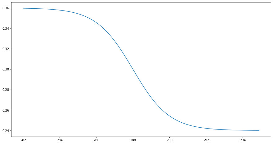
Task 5: In this parameterisation, the albedo is solely a function of mean temperature. As a non-linear function we assume a sigmoid function with
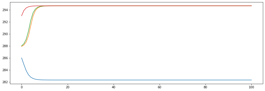
Run the energy balance model for 100 years with four different initial conditions for T(0)=286.0, 287.9, 288.0, and 293.0 K, while fixing the other parameters to \(C_w\)= 2\(\cdot10^8\) J/(m\(^2 \cdot\) K) and \(\tau_{mean}\)=0.608.
What can be said about the state of equilibrium?
# Import some modules which are used in the function
import random         # Module to generate random number
import numpy as np    # Numpy


def ebm_ice_albedo(T0, Q=341.3, Cw=10e8, alpha=0.3, tau=0.64, years=100):
    ''' This is a simple Energy Balance Model including ice-albedo feedback.'''

    # Create result arrays (numpy) filled with zeros
    # Ts stores the temperature values, years the years since the beginning of
    # the simulation
    Ts    = np.zeros(years+1)
    Years = np.zeros(years+1)

    # Timestep in seconds (time step is 1 year)
    dt = 60*60*24*365                  # convert days to seconds

    # Initial and boundary conditions
    # Set the first value in the Ts to the initial condition
    Ts[0] = T0

    # Integration over all years
    for n in range(years):
        # Parametrization of albedo. The albedo is a function of temperature.
        alpha_adapt = alpha * (1 - 0.2 * np.tanh(0.5*(Ts[n]-288)))
        # Store the number of iterations in the Years array
        Years[n+1] = n+1
        # Store the new temperature value in Ts
        Ts[n+1] = step_forward( Q, Ts[n], Cw, alpha_adapt, tau, dt )

    # Return both the temperature and year array
    return Years, Ts
# Plot the albedo function
# Plot the albedo function
# Create an array containing the temperature range from 282 K to 295 K
T_range = np.arange(282,295,0.1)

# Plot the albedo function
plt.figure(figsize=(15,8))
plt.plot(T_range, 0.3 * (1 - 0.2 * np.tanh(0.5*(T_range-288))));
# Run the simulations and plot the results
# Run several ice-albedo feedback simulations with different initial conditions
yrs, Ts286 = ebm_ice_albedo(286.0, Q=342, Cw=2*10**8, alpha=0.30, tau=0.608, years=100)
yrs, Ts287 = ebm_ice_albedo(287.9, Q=342, Cw=2*10**8, alpha=0.30, tau=0.608, years=100)
yrs, Ts288 = ebm_ice_albedo(288.0, Q=342, Cw=2*10**8, alpha=0.30, tau=0.608, years=100)
yrs, Ts293 = ebm_ice_albedo(293.0, Q=342, Cw=2*10**8, alpha=0.30, tau=0.608, years=100)

# Plot the result
fig, ax = plt.subplots(1,1,figsize=(15,5))
ax.plot(yrs, Ts286); ax.plot(yrs, Ts287); ax.plot(yrs, Ts288); ax.plot(yrs, Ts293);
Extend the model with a simple ice/land use albedo parameterisation. (linear version)
Task 6: In this parameterisation, the albedo is solely a function of mean temperature. We assume a simple linear relation according to
with \(T_i\)=273 K, and \(T_g\)= 292 K. Run the energy balance model for 100 years with four different initial conditions for T(0)=286.0, 287.9, 288.0, and 293.0 K, while fixing the other parameters to \(C_w\)= 2\(\cdot10^8\) J/(m\(^2 \cdot\) K), and \(\tau_{mean}\)=0.608, \(a_i\)=0.6, and \(a_g\)=0.2.
What can be said about the state of equilibrium?
import random
import numpy as np
import matplotlib.pyplot as plt


def ebm_ice_albedo_2(T0, Q=341.3, Cw=10e8, alpha=0.3, tau=0.608, years=100):
    # Write your code here
    pass
# Run the simulations and plot the results
Task 7: Determine the equilibrium climate sensitivity (ECS) and the feedback factor for the simulation from Task 5 using T(0)=289 K. (sigmoid albedo parametrisation)
import random
import numpy as np
import matplotlib.pyplot as plt


def ebm_ice_albedo_stochastic_ECS(T0, Q=341.3, Cw=10e8, alpha=0.3, tau=0.64, years=100):
    ''' This is a simple Energy Balance Model with a random transmissivity and
    ice-albedo feedback.'''

    # Timestep in seconds (time step is 1 year)
    dt = 60*60*24*365                  # convert days to seconds

    # Create result arrays (numpy) filled with zeros
    # Ts stores the temperature values, Years the years since the beginning of
    # the simulation, netQ the net radiation flux, and dT the temperature change
    Ts    = np.zeros(years+1) # Temperature
    netQ  = np.zeros(years)   # Net radiation flux at the tropopause
    dT    = np.zeros(years)   # Temperature change
    Years = np.zeros(years+1) # Years since simulation start

    # Initial and boundary conditions
    Ts[0] = T0

    # Integrate over all years
    for n in range(years):
        # Calculate the albedo value
        alpha_adapt = alpha * (1 - 0.2 * np.tanh(0.5*(Ts[n]-288)))
        alpha_adapt =0.3
        # Generate a random transmissivity
        tau_rnd = random.normalvariate(tau,tau*0.01)
        # Store the interation (year)
        Years[n+1] = n+1
        # Calculate the new tempeature
        Ts[n+1] = step_forward(Q, Ts[n], Cw, alpha_adapt, tau, dt)

        # Store the net radiation flux at the tropopause ASR-OLR
        netQ[n] = ASR(Q, alpha_adapt) - OLR(Ts[n], tau)

        # Store the temperature change between the current and previous step
        dT[n] = Ts[n] - Ts[0]

    # Return all result arrays
    return Years, Ts, dT, netQ
# Run the simulations and plot the results
yrs, Ts, dT, netQ = ebm_ice_albedo_stochastic_ECS(289, Q=342, Cw=2*10**8, \
                                                     alpha=0.30, tau=0.608, years=50)
# Create subplots
fig, (ax1, ax2) = plt.subplots(1,2,figsize=(20,6))

# Temperature time series
ax1.plot(yrs, Ts)

# Create a scatter plot: temperature change vs. net radiation flux
ax2.scatter(dT[1:], netQ[1:])

# Fit a regression line to the scatter plot
m, b = np.polyfit(dT[1:], netQ[1:],1)

# Add regression line to scatter plot
x = np.arange(0,np.max(dT),0.1)
ax2.plot(x, m*x+b)
ax2.axline((0,0),(1,0), linewidth=2, color='gray')
ax2.scatter(-b/m,0, s=90)


# Calculate the ECS from the regression line and print the result
print('The ECS is {:.2f} ºC'.format(-b/m))
print('The feedback factor is {:.2f}, which implies a negative feedback'.format(-m/b))
The ECS is -0.32 ºC
The feedback factor is -3.08, which implies a negative feedback

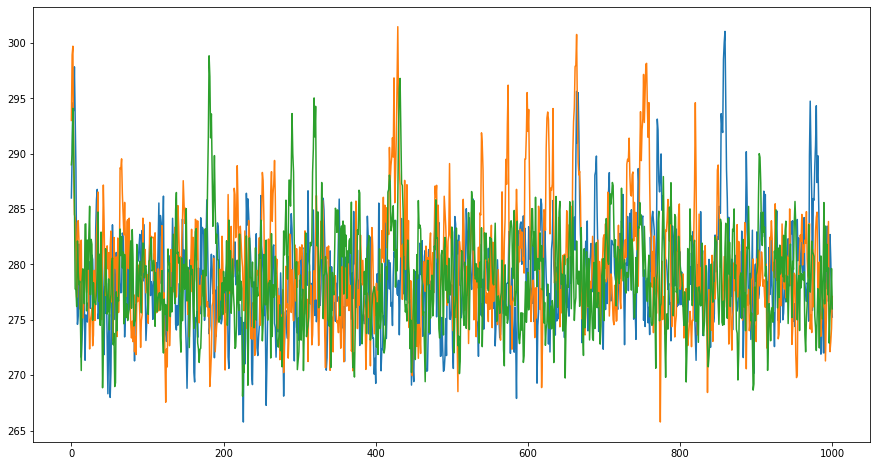
Task 8: Repeat the simulation from Task 5 (sigmoid function for albedo) with T(0)=289 K, but again sample the transmissivity from a normal distribution with a standard deviation of 10%.
What special feature can now be observed? What conclusions can be inferred regarding the prediction of weather and climate?
# Import some modules which are used in the function
import random         # Module to generate random number
import numpy as np    # Numpy


def ebm_ice_albedo_stochastic(T0, Q=341.3, Cw=10e8, alpha=0.3, tau=0.64, years=100):
    ''' This is a simple Energy Balance Model including ice-albedo feedback.'''

    # Create result arrays (numpy) filled with zeros
    # Ts stores the temperature values, years the years since the beginning of
    # the simulation
    Ts    = np.zeros(years+1)
    Years = np.zeros(years+1)

    # Timestep in seconds (time step is 1 year)
    dt = 60*60*24*365                  # convert days to seconds

    # Initial and boundary conditions
    # Set the first value in the Ts to the initial condition
    Ts[0] = T0

    # Integration over all years
    for n in range(years):
        # Parametrization of albedo. The albedo is a function of temperature.
        alpha_adapt = alpha * (1 - 0.2 * np.tanh(0.5*(Ts[n]-288)))

        # Sample the transmissivity from a normal distribution with a standard deviation of 10%
        tau_rnd = random.normalvariate(tau, tau*0.1)

        # Store the number of iterations in the Years array
        Years[n+1] = n+1
        # Store the new temperature value in Ts
        Ts[n+1] = step_forward( Q, Ts[n], Cw, alpha_adapt, tau_rnd, dt )

    # Return both the temperature and year array
    return Years, Ts
# Plot the results
yrs, Ts286 = ebm_ice_albedo_stochastic(286, Q=342,
                                       Cw=2*10**8, years=1000)

yrs, Ts293 = ebm_ice_albedo_stochastic(293, Q=342,
                                       Cw=2*10**8, years=1000)

yrs, Ts289 = ebm_ice_albedo_stochastic(289, Q=342,
                                       Cw=2*10**8, years=1000)

fig, ax = plt.subplots(1,1,figsize=(15,8))
ax.plot(yrs, Ts286)
ax.plot(yrs, Ts293)
ax.plot(yrs, Ts289)

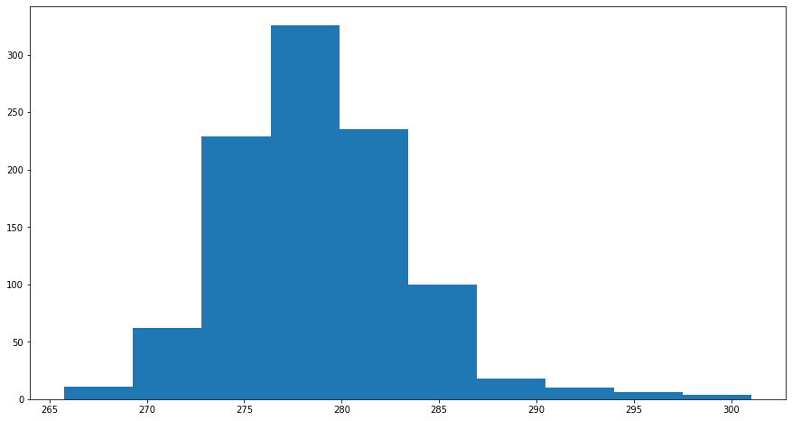
fig, ax = plt.subplots(1,1,figsize=(15,8))
plt.hist(Ts286)
(array([ 11.,  62., 229., 326., 235., 100.,  18.,  10.,   6.,   4.]),
 array([265.76944007, 269.29649473, 272.82354939, 276.35060405,
        279.8776587 , 283.40471336, 286.93176802, 290.45882268,
        293.98587733, 297.51293199, 301.03998665]),
 <BarContainer object of 10 artists>)
# Make more plots to illustrate the characteristics of the time series
